3.2 Sorting Algorithms

Sorting is a common problem in computer science. Not only is a sorted list useful in itself, but sorted lists often enable other algorithms, such as binary search, to work.

This brings up the question: How do you sort a list? Perhaps the most intuitive way is to find the minimum value in the list, and then move that to the first index. Then, find the next smallest value and move it to the second index. Then, keep finding the next smallest value and moving it to the next index until the list is sorted.

This is called Selection Sort.

Selection Sort

Many of you probably have used selection sort before in some way or another. Here’s an example implementation of this.


def selection_sort(lst):
    for i in range(len(lst)):
        min_value = lst[i]
        min_val_idx = i
 
        # find the new minimum value and its idx
        for x in range(i, len(lst)):
            if lst[x] < min_value:
                min_value = lst[x]
                min_val_idx = x
 
        # swap the minimum value with the value at the current idx
        lst[i], lst[min_val_idx] = min_value, lst[i]
    return lst
 
 
test1 = [3, 12, 7, 2, 0, 3]
test1 = selection_sort(test1)
print(test1)  # [0, 2, 3, 3, 7, 12]
 
test2 = [-23, 0, 72, -33, 11, 6, 2, -5, -9, 10, -1]
test2 = selection_sort(test2)
print(test2)  # [-33, -23, -9, -5, -1, 0, 2, 6, 10, 11, 72]
 
test3 = [i for i in range(1000, -1, -1)]
test3 = selection_sort(test3)  # [0, 1, 2, 3, 4, 5, 6, 7, 8, 9, 10, ...]
print(test3)

View code on GitHub.

Selection Sort - Pros and Cons

Although Selection Sort is definitely intuitive, it’s also not that efficient. Its runtime is O(n^2) since you have to traverse the array one time for each iteration. So, let’s talk about some less intuitive but faster methods to sort a list

Quicksort

Quick sort is a very famous sorting algorithm, namely for its speed. Especially in smaller lists, quicksort is sometimes twice or three times as fast as other sorting algorithms like bubble sort or heap sort. Quick sort is a “divide and conquer” algorithm, so it is easiest to implement with recursion. Let’s put ourselves in the shoes of someone trying to develop a really fast sorting algorithm and “discover” quick sort.

Let’s start with the following list: my_list = [43, 192, 234, 12, 3, 89, 78]

Let’s just take the last number in the list, 78, and put all of the elements smaller than 78 to the left, and all of the numbers larger than 78 to the right. We don’t care about whether the numbers to the left and right are ordered, just put it to the left or right side. If we do that, then our new list would look something like this:

my_list = [43, 3, 12, 78, 234, 192, 89] green - numbers SMALLER than 78 purple- numbers LARGER than 78

In this case, we have 3 numbers to the left of 78 and 3 numbers to the right. The list is obviously not sorted yet, because the areas in green and purple are not sorted. However, notice that the position of 78 doesn’t change even if the two regions WERE sorted. my_list = [43, 3, 12, 78, 234, 192, 89] sorted_list = [3, 12, 43, 78, 89, 192, 234] 78 is in the same place because the number of elements to the left and right don’t change even if they are sorted. Thus, you could say 78 is sorted, or we know it’s position if the entire list WAS sorted.

Let’s call this process of putting elements smaller than 78 to the left and elements larger than 78 to the right partitioning. And let’s call 78 the pivot, the element that we use as a reference to move other elements to the left or right side. Note that the pivot doesn’t need to have the left and right regions be the same size. We could have picked any other element to be the pivot. As an example, we can also pivot around 89, shown below. my_list = [43, 3, 78, 12, 89, 234, 192]

Before implementing quick sort, let’s just create a function that takes in a list and an index, and partitions the list with the pivot as the element with the index provided. There are many ways of doing this, but below is one approach.


def partition(arr, pi):
   """
   partition takes some pivot index (pi), and puts all of the items 
   smaller than pivot to the left, and all of the items larger than 
   pivot to the right,
  
   in doing so we put pivot in the same spot as if the entire list was
   sorted
 
   note: this is only one way of doing it
   """
   # moves pivot to the end of the list so it doesn't get in the way
   arr[-1], arr[pi] = arr[pi], arr[-1]
 
   i = 0 # i is initialized to be the left side of our list
 
   for j in range(len(arr)):
       # if j is smaller than the pivot, arr[j] is smaller than the pivot,
       # so we want to move it to the left
       if arr[j] < arr[-1]:
           # swaps arr[j] and arr[i], so arr[j] is at the left side of the list
           arr[i], arr[j] = arr[j], arr[i]
           i += 1
   # move the pivot from the end to the correct location
   arr[i], arr[-1] = arr[-1], arr[i]

Now that we have a partition function implemented, we can really easily create quick sort.

Let’s quickly look back at our partitioned list. my_list = [43, 3, 12, 78, 234, 192, 89] Notice that if we perform another partition in the green area (let’s partition off of the last element, 12) again, we once again find the correct location of 12, and we have two new areas to the left and right again. Notice that these new areas are only one element in size. my_list = [3, 12, 43, 78, 234, 192, 89] If they are only one element in size, we know that they must be sorted correctly. Thus, we can say that after partitioning the left side of 78, we sorted the entire left side.

If we partition the right side of 78 now (again, partitioning off of the last element, 89), we get the following. my_list = [3, 12, 43, 78, 89, 234, 192] In this case, we don’t have a left side of 89 because there are no elements, and a region of 2 elements on the right side of 89. Because the region is 2 elements long, we can’t necessarily say they are sorted yet, but we can just take that region and partition it again until it IS sorted. After partitioning the purple region, we have a fully sorted list below. my_list = [3, 12, 43, 78, 89, 192, 243]

In this way, we can partition the list, and then repeatedly partition the left and right side of each partition over and over again until the whole list is sorted. In order to make our partition algorithm work on specific regions of the list, we need to change our partition algorithm like so:


def partition(arr, low, high):
   # Note: always partitions with the last element as the pivot
 
   i = low # i is initialized to be the left side of our list
 
   for j in range(low, high):
       # if j is smaller than the pivot, arr[j] is smaller than the pivot,
       # so we want to move it to the left
       if arr[j] < arr[high]:
           # swaps arr[j] and arr[i], so arr[j] is at the left side of the list
           arr[i], arr[j] = arr[j], arr[i]
           i += 1
   # move the pivot from the end to the correct location
   arr[i], arr[high] = arr[high], arr[i]

In our function, low and high are the first and last indexes of the region that you are partitioning.

Now we need to just change the partition function to recursively call itself on the left and right side of each partition, as well as rename it to quick sort.


def quicksort(arr, low, high):
   # Note: always partitions with the last element as the pivot
 
   i = low # i is initialized to be the left side of our list
 
   for j in range(low, high):
       # if j is smaller than the pivot, arr[j] is smaller than the pivot,
       # so we want to move it to the left
       if arr[j] < arr[high]:
           # swaps arr[j] and arr[i], so arr[j] is at the left side of the list
           arr[i], arr[j] = arr[j], arr[i]
           i += 1
   # move the pivot from the end to the correct location
   arr[i], arr[high] = arr[high], arr[i]
   
   quicksort(arr, low, i - 1) # left side of the pivot
   quicksort(arr, i + 1, high) # right side of the pivot

View code on GitHub.

Quicksort - Pros and Cons

Pros - the average runtime is O(nlog(n)). This is often faster than other algorithms.

Cons - Quicksort is inconsistent. In worst case scenarios, the pivot quicksort uses is always either the greatest or smallest element of the partition, in which case the time complexity is O(n^2). For a much more stable sorting algorithm in terms of speed, look towards merge sort.

Mergesort

Mergesort is another less intuitive algorithm, but it is reliable and efficient.

Mergesort, like quicksort, is a recursive sorting method. Because it is recursive, it’s important that we have a base case for determining when we can say that an array is sorted. So, we take the same assumption we made in quicksort and say that an array is already sorted if the requested portion of it has a length of 0 or 1 (because any array of length 0 is sorted, and any 1 number by itself is also sorted).

Mergesort Logic

If the requested portion of the list to sort has a length of 0 or 1, just return that portion. If not, then break down the portion of the list into two halves Sort the first half using recursive call to mergesort Sort the second half using recursive call to mergesort Finally, merge the parts into a sorted list and return that

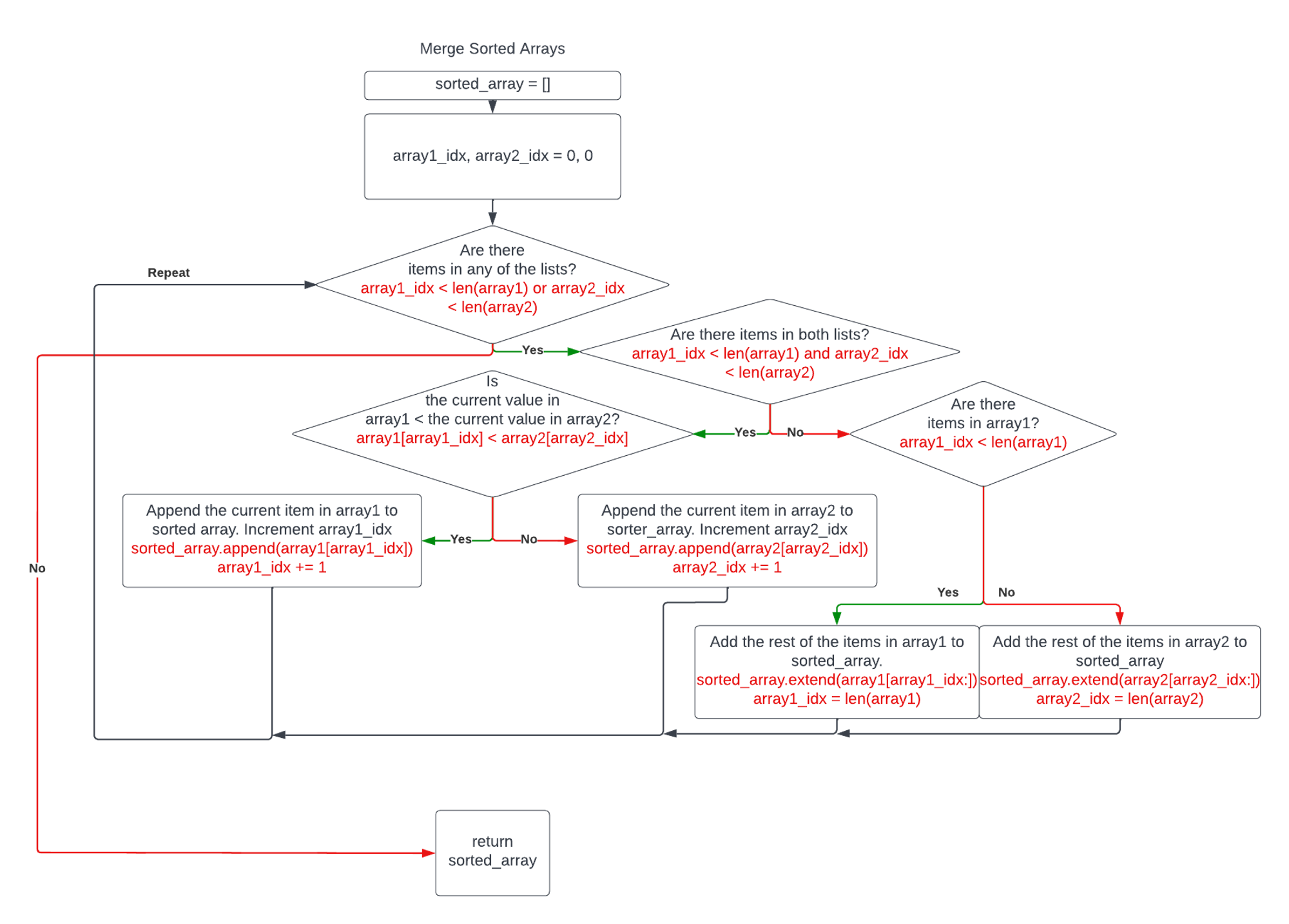
This might leave you wondering - “How does this even work?”. Well, the key to this sorting method working is the merging of the sorted parts. The logic in merging two sorted arrays is simple. We show the merging logic in the following diagram.

Merging sorted arrays

Mergesort demo

Now that we know how to merge arrays, we can see mergesort in action. It first breaks down the array into arrays of length 1. It then merges the arrays, creating a sorted array.

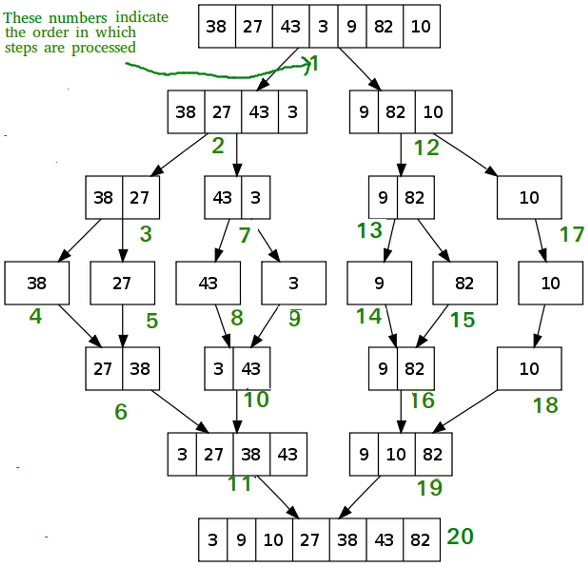
Image courtesy of Geeks for Geeks

Python Implementation


def mergelists(lst1, lst2):
    idx1 = 0
    idx2 = 0
    ret = []

    # while either one has unused items
    while idx1 < len(lst1) or idx2 < len(lst2):
        # both lists still have items
        if idx1 < len(lst1) and idx2 < len(lst2):
            if lst1[idx1] < lst2[idx2]:
                ret.append(lst1[idx1])  # add the item from lst1
                idx1 += 1  # increment our idx in lst1
            else:  # lst2[idx2] <= lst1[idx1]
                ret.append(lst2[idx2])  # add the item from lst2
                idx2 += 1  # increment our idx in lst2

        # only one list still has items
        elif idx1 < len(lst1):  # if only lst1 still has items
            ret.extend(lst1[idx1:])  # add the rest of this list
            idx1 = len(lst1)
        elif idx2 < len(lst2):  # if only lst2 still has items
            ret.extend(lst2[idx2:])  # add the rest of this list
            idx2 = len(lst2)

    return ret


def mergesort(lst):
    # "base case" where the list is just 0 or 1 item(s).
    # In this case, we can say it is already sorted and just return it.
    if len(lst) <= 1:
        return lst

    # if it's not just 1 or 0 item(s), then follow mergesort logic
    middle_idx = len(lst) // 2  # we want an integer, so use //
    first_half = mergesort(lst[:middle_idx])  # sort the first half
    second_half = mergesort(lst[middle_idx:])  # sort the second half
    return mergelists(first_half, second_half)  # merge the two sorted halves


print(mergesort([5, 4, 3, 2, 1]))
print(mergesort([i for i in range(99, -1, -1)]))

View code on GitHub.

Mergesort - Pros and Cons

Pros - Its worst-case, best-case, and average runtime are all O(nlog(n)). This is amazingly stable and reliable for a sorting algorithm.

Cons - It is less space efficient because it creates new lists.

Practice

Selection Sort

Let's implement selection sort! There are 4 easy steps to follow in order to implement it. 1. Create a loop through iterate through the list. 2. Create an inner loop that iterates from the outer index + 1 to the end of the list. 3. Compare the element at the outer index to the element at the inner index. 4. If the element at the outer index is larger than at the inner index, swap the 2 elements.

Template code is provided for you.

💻 Template Code

✅ Solution Code

Merge Sort

Let's implement merge sort! Template code is provided, so follow the instructions in the comments and fill in the blanks.

💻 Template Code

✅ Solution Code

Quick Sort

Let's implement quick sort! Template code is provided, so follow the instructions in the comments and fill in the blanks.

💻 Template Code

✅ Solution Code

Previous Section

1️⃣

3.1 Search Algorithms

Next Section

3️⃣

3.3 Pathfinding Algorithms

⚖️

Copyright © 2021 Code 4 Tomorrow. All rights reserved. The code in this course is licensed under the MIT License. If you would like to use content from any of our courses, you must obtain our explicit written permission and provide credit. Please contact classes@code4tomorrow.org for inquiries.