The Cost Function
To determine which line fits the data most optimally, we first need to define the criteria in which we evaluate a line. In machine learning, this is called the cost function. The cost function will compare a given line with the data and output a number that represents how well the line fits it.
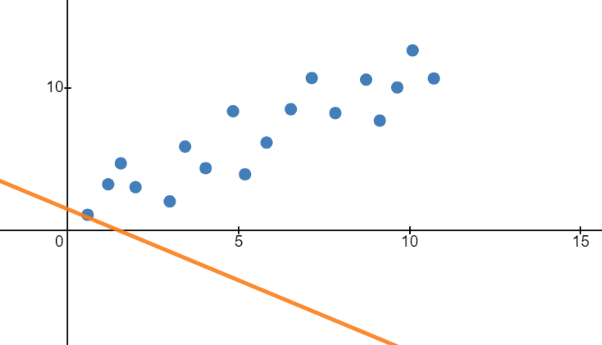
A line that poorly fits the data will have a very high cost function:
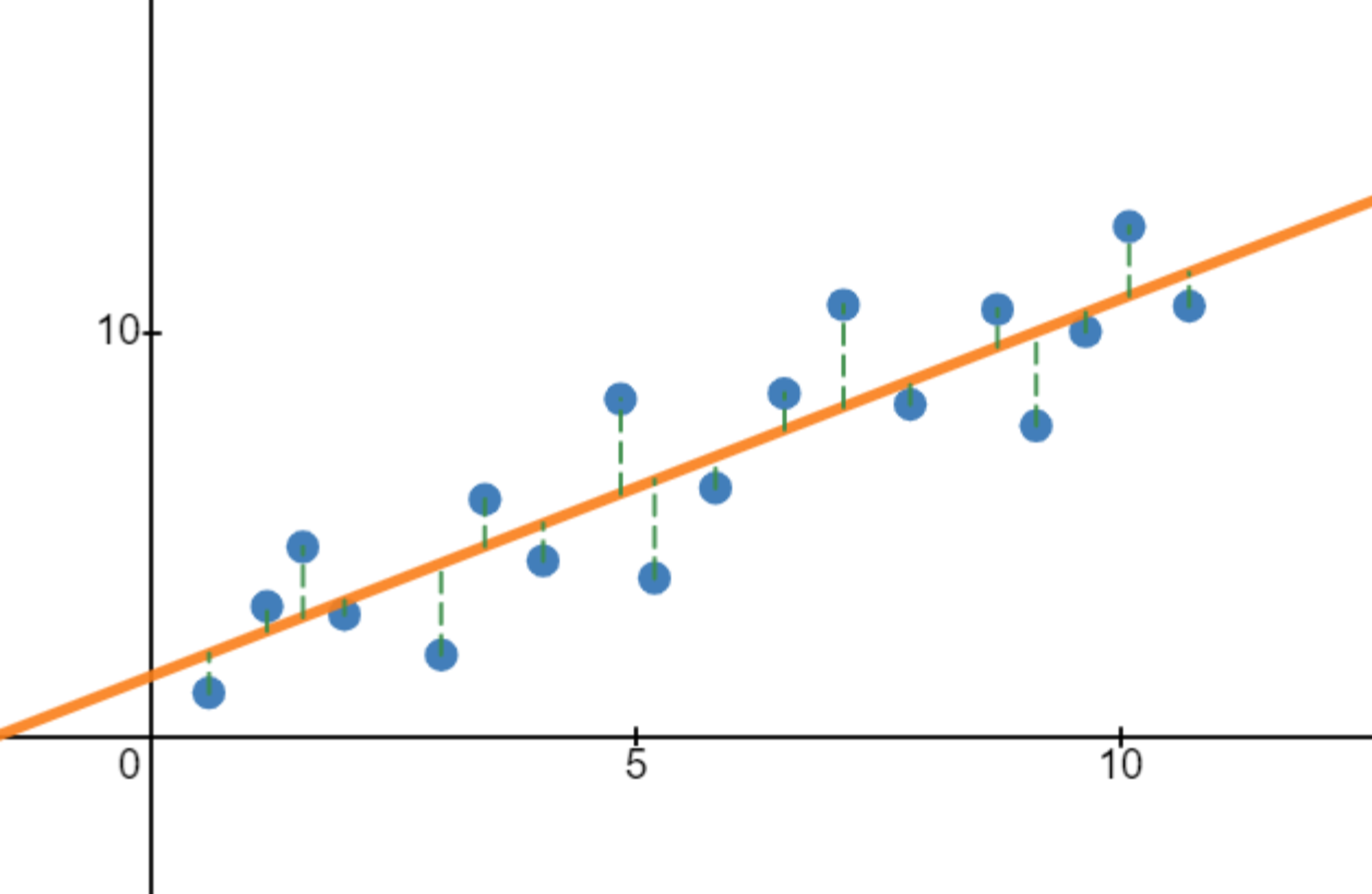
Whereas a line that fits the data well will have a low cost function:
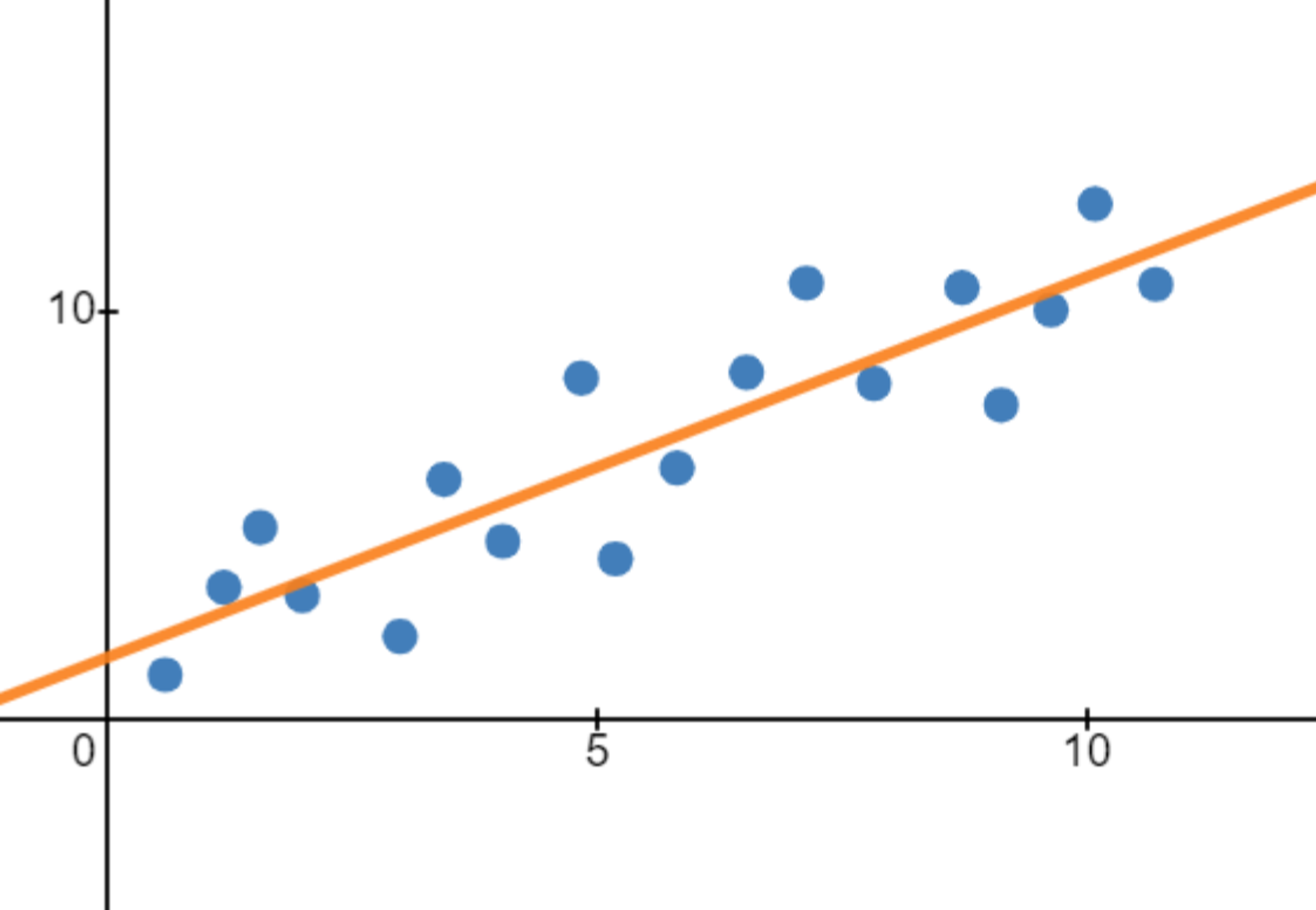
So how can we go about creating a cost function for linear regression? The most intuitive approach is to find the average vertical distance between the line and each data point:
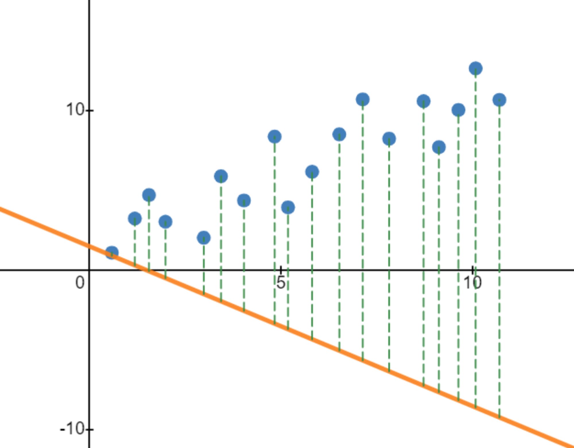
As you can see, the vertical distances are on average pretty large, which is why the first line has a rather big cost function. On the other hand, the vertical distances are pretty small on average for the second line, leading to a low cost function:
Mathematically, we can define the cost function we've just discussed as follows:
Here, is the number of data points there are, is the y-value of the -th point, and is the y-value of the line at the x-value of the -th point. By finding the sum of for every single data point, we sum up all of the distances between the points and the line. Then, by dividing that sum by we find the average distance between each point and the line — hence the cost function we originally wanted.
While this cost function is probably the most intuitive and seemingly the most effective, statisticians have found the following cost function to be even more effective for linear regression:
By squaring instead of taking its absolute value, we punish the model a lot more for very large distances between each point and the line. Thus, a line that optimizes this cost function will ensure a good fit by prioritizing minimizing especially large errors.
We will be using the above cost function for linear regression. That means that when we try fitting a line to any 2-dimensional dataset, we'll be looking for a line such that is minimized.
Gradient Descent
To actually find a line that minimizes the cost function, we can use a method called gradient descent. Gradient descent is an incredible optimization method courtesy of statistics.
Let's say that we graphed our cost function for every possible value of with a constant :
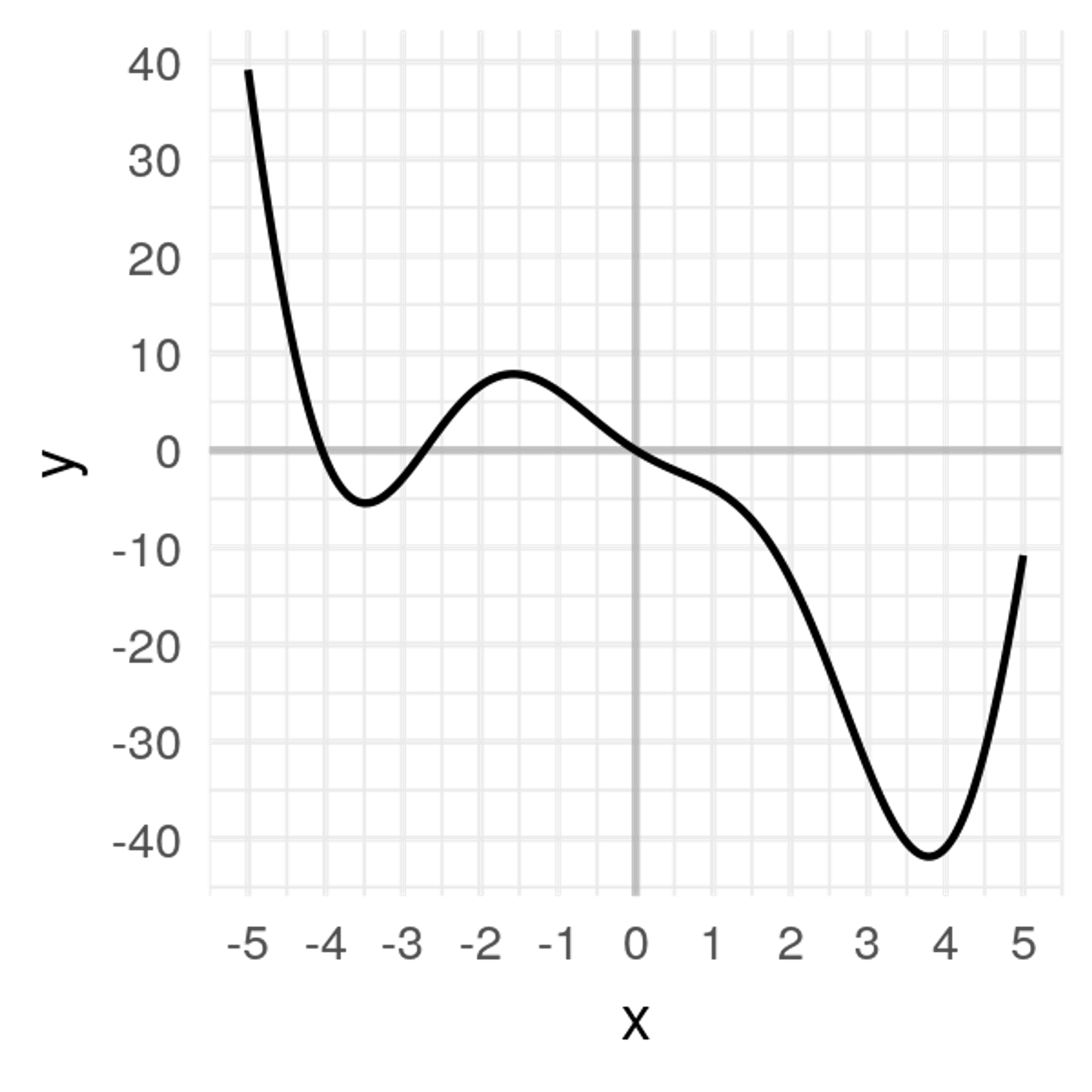
With linear regression, our cost function won't actually look like this when graphed versus , but let's just go with this graph for the sake of our example. Now, we're going to try to find the minimum value of the cost function procedurally.
We will use the term to represent the slope of the graph of the cost function at a particular point and to represent what we call the learning rate. The learning rate represents step size. You'll see what that means in a minute.
Now, let's begin gradient descent:
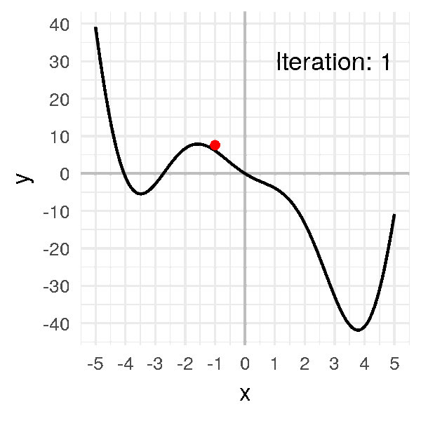
Step 1
Start with a random x-value.
Step 2
For this random value, calculate the slope (or derivative) of the cost function there. This might be a bit of a strange concept — calculating the slope at one point — but this can be done by calculus. This is .
Step 3
Next, we will update using the following update rule:
If the slope at the point we're at is steeper, we will move down the slope with a bigger step size. In contrast, if it's not as steep, we will move with a smaller step size.
In this update rule, is a constant that represents the learning rate, which essentially is a multiplier for how big the steps we take are. With a bigger value of , all steps we take will be made larger. In turn, the model can learn faster. However, a value of that's way too big can cause the model to make such a big step that it misses the minimum. A smaller value of makes the model learn slower, however it ensures that we will find the minimum.
Step 4
We then repeat Steps 2-4 again and again until we reach a local minimum.
We will be applying the process of gradient descent to minimize the cost function for the linear regression model, which essentially determines how close the model is to representing the data. By minimizing the cost function, we'll find the optimal for extra-simple regression ().
Put together, this is what gradient descent looks like:
As you can see, we can think of gradient descent almost like a ball rolling down a curved surface!
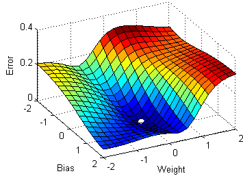
Since this gradient descent method only calculates the optimal value for , you may be wondering how we would calculate the optimal value for all parameters. It turns out that this process is essentially identical, except that we'll be dealing with cost function graphs with bigger dimensions. In the case for linear regression, there are two parameters and . Since we want to create a graph with these two parameters and the cost function, our graph will be three dimensional. Here's what gradient descent could look like:
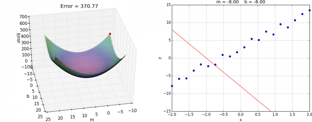
We can also visualize gradient descent and linear regression together (this visualization uses for and for ):
Ordinary Least Squares
We won't go into the mechanics of Ordinary Least Squares works, but effectively it is a direct solution to the optimization problem for Simple Linear Regression. That means there's an equation for the optimal value of each parameter, which just needs to be calculated.
At any rate, within this course, we'll be using a library to deal with all of this stuff, so don't worry about the actual working of OLS.
Now that we've understood Gradient Descent and OLS, we'll go to work on our first implementation of Linear Regression.
Links
Analytics Vidhya - (This article gets a bit more technical, Calculus background may be suggested)
Videos: 3Blue1Brown
Copyright © 2021 Code 4 Tomorrow. All rights reserved.
The code in this course is licensed under the MIT License.
If you would like to use content from any of our courses, you must obtain our explicit written permission and provide credit. Please contact classes@code4tomorrow.org for inquiries.
